Import standard modules:
import numpy as np
import matplotlib.pyplot as plt
%matplotlib inline
from IPython.display import HTML
HTML('../style/course.css') #apply general CSS
Import section specific modules:
import ipywidgets
from IPython.display import Image
HTML('../style/code_toggle.html')
1.10 The Limits of Single Dish Astronomy
In the previous section ➞ of this chapter we introduced the concepts and historical background of interferometry. Earlier in the chapter we presented some of the basic astrophysical sources which emit in the radio spectrum. In this section we will try to answer why we need to use interferometry in radio astronomy. A related question we will try to answer is why we can not just use a single telescope as is done in traditional optical astronomy.
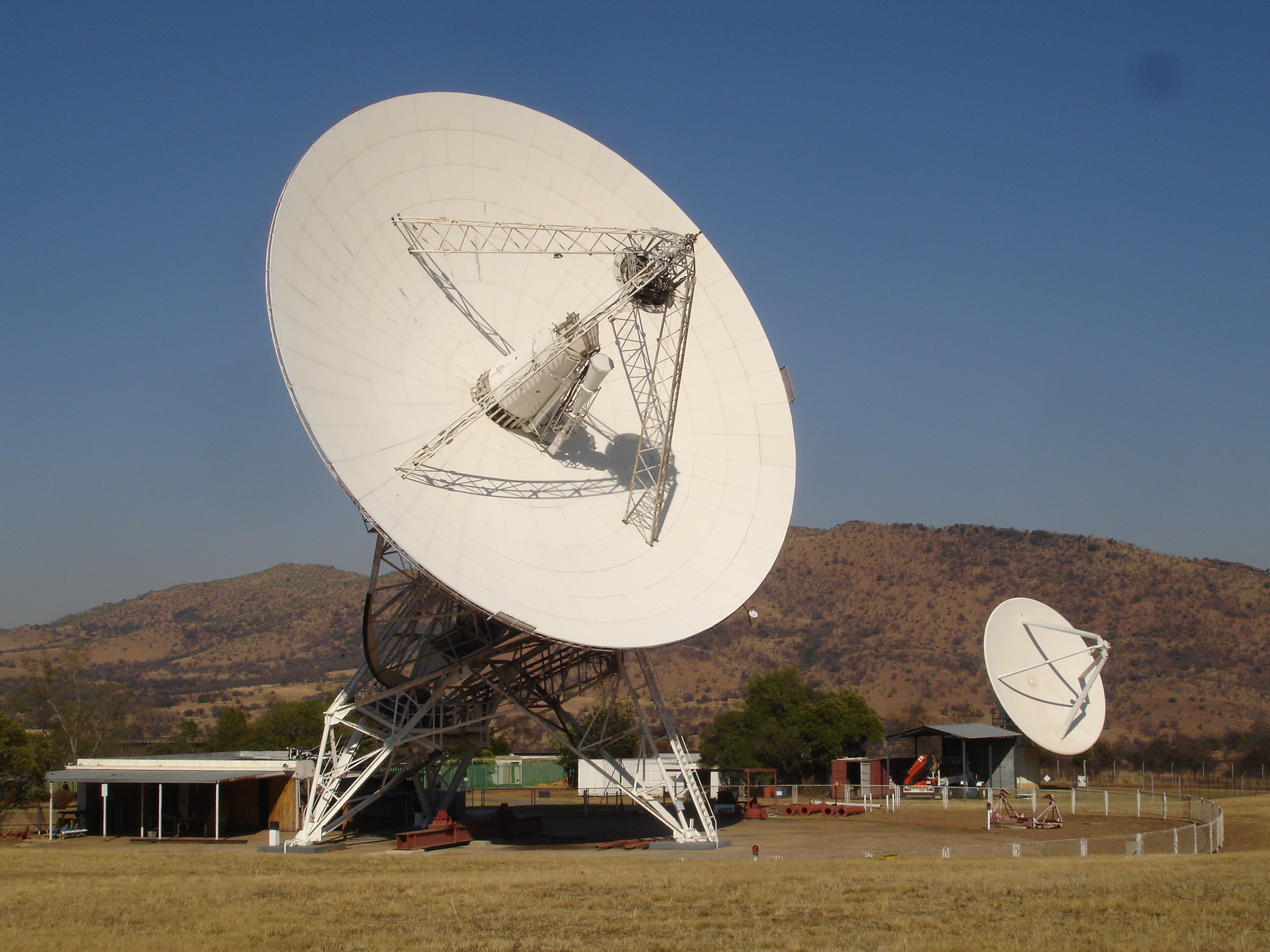
Single telescopes are used in radio astronomy, and provide complimentary observational data to that of interferometric arrays. Astronomy with a single radio telescope is often called single dish astronomy as the telescope usually has a dish reflector (Figure 1.10.1). This dish is usually parabolic, but other shapes are used, as it allows for the focusing of light to a single focal point. At the focal point a reciever is placed - among other instruments this could be a camera in the optical, a bolometer in the far-infrared, or an antenna feed in the radio. Instead of a single dish telescope, a more general term would be a single element telescope which can be as simple as a dipole (Figure 1.10.2). An interferometric array (Figure 1.10.3) is used to create a synthesized telescope as it is considered a single telescope synthesized out of many elements (each element is also a telescope, it can get even more confusing).
Image(filename='figures/hart_26m_15m_2012-09-11_08511.jpg')

Figure 1.10.1: 26 meter dish at HartRAO, South Africa used for single dish observations and as part of interferometric VLBI networks. Credit: M Gaylard / HartRAO⤴
Image(filename='figures/kaira_lba_element.jpg')

Figure 1.10.2: LOFAR LBA dipole element. Credit: KAIRA/D. McKay-Bukowski⤴
Image(filename='../5_Imaging/figures/2013_kat7_20.jpg')

Figure 1.10.3: Inner 5 dishes of KAT-7, a 7 element interferometric array located in South Africa which can be combined into a single synthesized telescope. Credit: SKA-SA⤴
Depending on the science goals of an expierment or an observatory different types of telescopes are built. So what is the main driver for building an interferometric array to create a synthesized telescope? It all comes down the resolution of a telescope which is related to the wavelength of light and the physical size of the telescope.
1.10.1. Aperture Diameter and Angular Resolution
If we consider a generic dish radio telescope, and ignoring blockage from feeds and structure and any practical issues, we can think of the dish as having a circular aperture. We will use the term 'primary beam' later in Chapter 7 to discuss this aperture in detail. Until then we can think of the dish aperture size as being the collecting area. The larger the aperture the more collecting area, thus the more sensitive (a measure of how well the telescope is able to measure a signal) the telescope. This is the same as in photography. Since we are modelling our simple telescope as a circle then the collection area $A$, or aperture size, is proportional to the diameter of the dish $D$.
$$A \propto D^2$$An additional effect of a larger aperture is an increase in the angular resolution of the telescope. That is the ability to differentiate between two source (say stars) which are separated by some angular distance. Using the Rayleigh criterion the angular resolution $\Delta \theta$ (in radians) of a dish of diameter $D$ is
$$\Delta \theta = 1.22 \frac{\lambda}{D},$$where $\lambda$ is the observing wavelength. Since light in the radio regime of the light spectrum has a longer wavelength as compared to optical light we can see that a radio telescope with the same collectiong area diameter as an optical telescope will have a much lower angular resolution.
The sensitivity of an telescope is directly proportional to the collecting area. The angular resolution of the telescope is inversely proportional to the aperture diameter. Usually, we want both high sensitivity and fine angular resolution, since we are interested in accurately measuring the strength of the signal and positions of sources. A natural way to improve both the sensitivity and angular resolution of a single telescope is to increase the collecting area.
The following table shows the angular resolution as a function of aperture diameter $D$ and observing wavelength for a single dish telescope.
| Telescope Type | Angular Resolution $\Delta \theta$ |
Visible $\lambda$ = 500 nm |
Infrared $\lambda$ = 10 $\mu$m |
Radio EHF $\lambda$ = 10 mm 30 GHz |
Radio UHF $\lambda$ = 1 m 300 Mhz |
|---|---|---|---|---|---|
| Amatuer | 0.8'' | 15 cm | 3 m | 3 km | 300 km |
| Automated Follow-up | 0.25'' | 50 cm | 10 m | 10 km | 100 km |
| Small Science | 0.12'' | 1 m | 21 m | 21 km | 2100 km |
| Large Science | 0.015'' (15 mas) | 8 m | 168 m | 168 km | 16800 km |
Table 1.10.1: Angular resolution of a telescope as a function of the aperture diameter $D$ and observing wavelength.
As we can see in Table 1.10.1, a radio telescope many orders of magnitude larger in diameter compared to an optical telescope is required to achieve the same angula resolution of the sky. It is very reasonable to build a 15 cm optical telescope, in fact they can be easily bought at a store. But a radio telescope, observing at 300 MHz, which has the same resolution (0.8 arcseconds) needs to have an aperture of 300 km! Now, this would not only be prohibitvely expensive, but the engineering is comepletely infeasible. As a matter of reference the largest single dish telescopes are on the order of a few hundred meters in diameter (see FAST in China, Arecibo in Puerto Rico). The following example shows how the diamter of a telescope varies as a function of observing wavelegth and desired angular resolution.
def WhichDiameter(wavelength=1., angres=(15e-3/3600)):
    """Compute the diameter of an aperture as a function of angular resolution and observing wavelength"""
    c = 299792458. #spped of light, m/s
    freq = c/(wavelength)/1e6 #
    D = 1.22 * wavelength/np.radians(angres) # assuming a circular aperture

    print '\n'
    print 'At a frequency of %.3f MHz (Lambda = %.3f m)'%(freq, wavelength)
    print 'the aperture diameter is D = %f m'%D
    print 'to achieve an angular resolution of %f degrees / %f arcmin / %f arcsec'%(angres, angres*60, angres*3600)
    print '\n'

w = ipywidgets.interact(WhichDiameter, angres=((15e-3/3600), 10, 1e-5), wavelength=(0.5e-6, 1, 1e-7))
1.10.2 Physical limitations of single dishes
There are certain physical limitations to account for when designing single dish radio telescopes. As an example, consider that, due to its limited field of view and the rotation of the earth, an antenna will have to track a source on the sky to maintain a constant sensitivity. In principle this can be achieved by mounting the antenna on a pedestal and mechnically steering it with a suitable engines. However, in order to maintain the integrity of the antenna, the control systems for these engines need to be incredibly precise. Clearly, this gets harder as the size of the instrument increases and will constitute a critical design point on the engineering side. This is true in the optical case as well, but it easier to manage as the telescope is physically smaller.
There is an upper limit on how large we can build steerable single dish radio telescopes. This is because, just like everything else, the metals that these telescopes are made out of can only withstand finite amounts of stress and strain before deforming. Perhaps one of the greatest reminders of this fact came in 1988 with the collapse of the 300 foot Green Bank Telescope ⤴ (see Figure 1.10.4). Clearly, large steerable telescopes run the risk of collapsing under their own weight. The 100 meter Green Bank Telescope (GBT) which replaced the 300 foot telescope is the largest steerable telescope in the world.
Larger single dish apertures can still be reached though. By leaving the reflector fixed and allowing the receiver at the focus to move along the focal plane (or along the caustic) of the instrument will mimic a slowly varying pointing in the sky (a so called steerable focus telescope). Indeed, this is how the Arecibo Observatory radio telescope (see Figure 1.10.5) operates. However, steerable focus telescopes come with limitations of their own (e.g. material cost and available space). In order to overcome these physical limations and acheive a higher angular resolution we must use interferometric arrays to form a synthesized telescope.
Image(filename='figures/gbt_300foot_telescope.jpg')

Figure 1.10.4a: 300 foot Green Bank Telescope located in West Virgina, USA during initial operations in 1962. Credit: NRAO⤴
Image(filename='figures/gbt_300foot_collapse.jpg')

Figure 1.10.4b: November, 1988, a day after the collapse of the 300 foot GBT telescope due to structural defects. Credit: NRAO⤴
Image(filename='figures/arecibo_observatory.jpg')

Figure 1.10.5: 300 m Arecibo Telescope lying in a natural cavity in Puerto Rico. The receiver is located in the white spherical structure held up by wires, and is repositioned to "point" the telescope. Credit: courtesy of the NAIC - Arecibo Observatory, a facility of the NSF⤴
1.10.3 Creating a Synthesized Telescope using Interferometry
Here we will attempt to develop some intuition for what an interferometric array is and how it is related to a single dish telescope. Before getting into the mathematics we will construct a cartoon example. A simple single dish telescope is made up of a primary reflector dish on a mount to point in some direction in the sky and a signal receptor at the focal point of the reflector (Figure 1.3.6a). This receptor, in the case of radio astronomy is an antenna, in optical astronomy the receptor is often a camera.
Basic optics tells us how convex lenses can be used to form real images of sources that are very far away. The image of a source that is infinitely far away will form at exactly the focal point of the lens, the location of which is completely determined by the shape of the lens (under the "thin lens" approximation). Sources of astrophysical interest can be approximated as being infinitely far away as long as they are at distances much farther away than the focal point of the lens. This is immediately obvious from the equation of a thin convex lens:
$$ \frac{1}{o} + \frac{1}{i} = \frac{1}{f}, $$where $i, ~ o$ and $f$ are the image, object and focal distances respectively. Early astronomers exploited this useful property of lenses to build the first optical telescopes. Later on concave mirrors replaced lenses because it was easier to control their physical and optical properties (e.g. curvature, surface quality etc.). Reflective paraboloids are the most efficient at focussing incoming plane waves (travelling on-axis) into a single locus (the focal point) and are therefore a good choice for the shape of a collector.
In our simple model the sky only contains a single astrophysical source, which is detected by pointing the telescope in its location in the sky.
Image(filename='figures/cartoon_1.png')

Figure 1.10.6a: A simple dish telescope which reflects incoming plane waves (red dashed) along ray tracing paths (cyan) to a receptor at the focal point of the parabolic dish.
Ignoring real world effects like aperture blockage and reflector inefficiencies, plane waves are focused to a single point using a parabolic reflector. At that focus if a signal receptor. We can imagine the reflector is made up of many smaller reflectors, each with its own reflection path. A single dish, in the limit of fully sampling the observing wavelength $\lambda$, can be thought of as being made up of enough reflectors of diameter $\lambda/2$ to fill the collecting area of the dish. In our simple example, we just break the dish into 8 reflectors (Figure 1.10.6b). This is in fact what is often done with very large telescopes when it is not feasible to build a single large mirror, such as in the W. M. Keck Observatory. At this point we have not altered the telescope, we are just thinking about the reflector as being made up of multiple smaller reflectors.
Image(filename='figures/cartoon_2.png')

Figure 1.10.6b: The dish reflector can be thought of as being made up of multiple smaller reflectors, each with its own light path to the focus.
Now instead of capturing all the signal at a single point, there is no reason we can not capture the signal at the smaller, individual reflector focus points. If that signal is captured, we can digitally combine the signals at the main focus point later (Figure 1.10.6c). This is the first trick of interferometry. Radio waves can be sufficiently sampled in time digital record the signals (this becomes more difficult at higher frequencies, and not possible in the near-infrared and higher). The cost is that a receptor needs to be built for each sub-reflector, and additional hardware is required to combine the signals. The dish optically combines the light, we are just doing the same digitally.
Image(filename='figures/cartoon_3.png')

Figure 1.10.6c: A receptor at each sub-reflector captures the light signals. To recreate the combined signal at the main receptor the signals are digitally combined.
The next leap is that there is no reason the sub-reflectors need to be set in the shape of a dish since the combination of the signal at the main focus is being done digitally. Since light travels at a constant speed then any repositioning of a sub-reflector just requires a time delay correction. So, we move each element to the ground, and construct a pointing system for each sub-reflector (Figure 1.10.6d). We now has an array of smaller single dish telescopes! By including the correct time delays on each signal the original, larger single dish telescope can be reconstructed. This digital operation is called beamforming and related to interferometry.
Image(filename='figures/cartoon_4.png')

Figure 1.10.6d: The sub-reflector elements of the original telescope are set on the ground with their own pointing systems. The original signal can be reconstructed digitally and by including the appropriate time delay for each telescope.
The beamforming opertation recombines all the signals into a single signal, with can be thought of as a single pixel camera. But, we can do better using a correlator which is a way of computing visibilities which are then used to form a image (Figure 1.10.6e), this will all be covered throughout the chapters that follow. But for now it is important to know that interferometric arrays have the advantage over single dish telescopes in that images can be generated instead of a single combined signal. The advantage is that much larger 'synthesized' telescopes can be constructed this compared to a single dish telescope. The correlator also allows for the creation of image over a beamformer at the cost of additional computing hardware.
Image(filename='figures/cartoon_5.png')

Figure 1.10.6e: By using correlator hardware instead of a beamformer an image of the sky can be created.
The next trick of interferometry is that we do not neccessarly need to sample the entire original dish (Figure 1.10.6f). We do lose sensitivity and, as will be discussed in later chapeters, spatial frequency modes, but by using only a subset of elements and understanding interferometry we can build synthesized telescopes that are many kilometers in diameter (e.g. MeerKAT) or as large as the Earth (e.g. VLBI netowrks). This is why radio interferometry can be used to produce the highest resolution telescopes in the world.
Image(filename='figures/cartoon_6.png')

Figure 1.10.6f: Radio interferometric arrays do not need to sample every location of the original telescope, this allows for large diameter 'synthesized' telescopes which can be larger than the diameter of Earth.
This simple example hides much of the detail and we have yet to discuss the limitations of interferometric arrays and synthesized telescopes. But, for the moment it is sufficient to think of interferometry as a method for overcoming the physical and engineering limations of build a single, massive telescope at the cost of additional digital hardware.
In this introductory section we have highlighted why we need multi-element instruments. Since radio observations are at a much longer wavelength (lower frequency) than those made in the visible, we would need much bigger radio telescopes to achieve the same angular resolution of optical telescopes. Array telescopes allow us to increase angular resolution and, by adding together the collecting areas of all the telescopes in the array, increase the sensitivity of the telescope. Because of the physical limitations involved in constructing very large single dish telescopes, it would be very difficult (and expensive) to achieve the same resolution and sensitivity with a single dish as with an array of telescopes. However, as we will see, interferometry introduces a number of additional challenges.
In the next section we will provide an overview of common interferometric arrays in use, the main science goals of the arrays, and future arrays in development.
Important things to remember
• A paraboloid reflector can be used to focus light from the far field to a single focal plane.
• The reflector mirror is an easier optical system to build and maintain compared to a transmitting lens.
• As we are dealing with EM waves, there is a *direct analogy between the properties of visible and radio telescopes*.
• In principle, an interferometer can be built by decomposing a single reflector instrument into smaller manageable pieces and by combining their signals in a specific manner.
• Conversely, a single reflector telescope can be interpreted as a continuous interferometer.
- reframe as aperture synthesis. resolution is important, but if that was all we wanted then we could just build beamformers, the real advantage is the imaging.